Interpolation to stations: ICON-CH2 wind gusts#

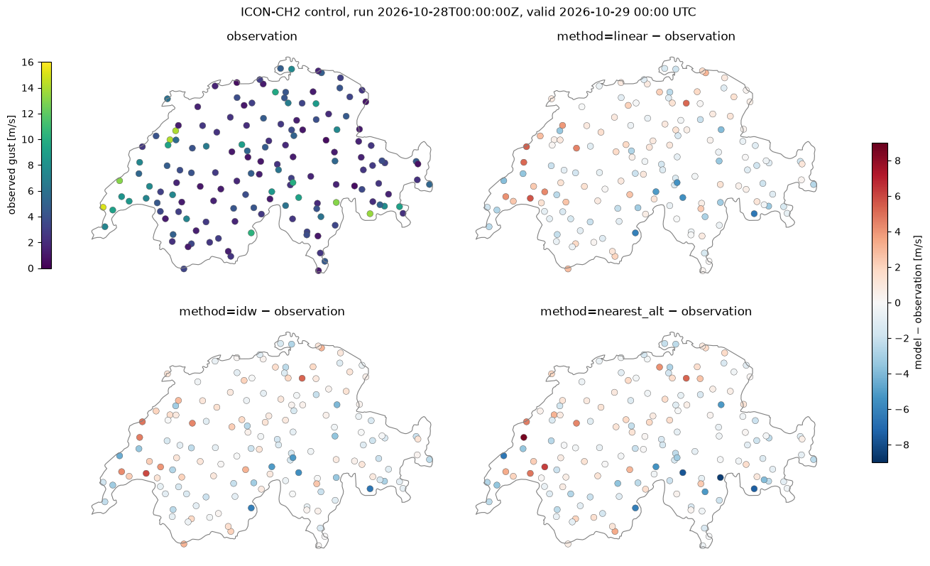
This example illustrates interp2poi() with three methods:

linear: linear interpolation on the triangulation of the source grid points;
idw: inverse distance weighting of the k nearest grid points, with weights d^(-weight_power);
nearest_alt: among the grid points within r_search grid spacings, the one with the most similar altitude. This suits wind, which depends strongly on the exposure of the site.

The hourly maximum 10 m wind gust (VMAX_10M) of the ICON-CH2 control forecast, on its native unstructured grid (about 2 km), is interpolated to the MeteoSwiss automatic weather stations measuring gusts, and compared with the observed hourly maximum gust.

Data: MeteoSwiss open data, CC BY 4.0, source: MeteoSwiss. Country borders: Natural Earth.

import contextlib
import datetime as dt
import io
import os
import time
import timeit
from collections.abc import Callable
from concurrent.futures import ThreadPoolExecutor
from functools import partial
from typing import Any

# import pyproj before earthkit.data to avoid a crash at exit (earthkit-data#1202)
import pyproj  # noqa: F401  # pylint: disable=unused-import
import eccodes_cosmo_resources

# ICON GRIB files need the COSMO definitions of ecCodes
os.environ["ECCODES_DEFINITION_PATH"] = str(eccodes_cosmo_resources.get_definitions_path())
os.environ["ECCODES_VERSION_CHECK_OFF"] = "1"
# grid_process data model (read at import): the SwissMetNet metadata columns give the POI labels and altitudes
os.environ["GRID_PROCESS__data_model__poi__coord_from"] = "station_abbr"
os.environ["GRID_PROCESS__data_model__poi__alt_from"] = '["station_height_masl"]'

import cartopy.io.shapereader as shpreader
import earthkit.data as ekd
import geopandas as gpd
import matplotlib.pyplot as plt
import numpy as np
import pandas as pd
import requests
import xarray as xr

import grid_process.grid_interp as gri
import grid_process.timeseries as tms

METHODS: dict[str, dict[str, Any]] = {
    "linear": {"method": "linear"},
    "idw": {"method": "idw", "k": 4, "weight_power": 2},
    "nearest_alt": {"method": "nearest_alt", "r_search": 1.7},
}

Stations and observations#

The stations measuring gusts are selected from the data inventory. Their metadata provide the coordinates and the altitude used by nearest_alt. Instead of renaming the metadata columns, the environment variables set in the setup cell adapt the grid_process data model: the station_abbr column becomes the poi coordinate of the output and station_height_masl gives the altitude. The observed hourly maximum gust (fkl010h1, 1 s peak) and VMAX_10M both refer to the hour ending at the valid time. The maps show the latest lead time with observations, taken from the files of the current day.

SMN_URL = "https://data.geo.admin.ch/ch.meteoschweiz.ogd-smn"
GUST = "fkl010h1"

inventory = pd.read_csv(f"{SMN_URL}/ogd-smn_meta_datainventory.csv", sep=";", encoding="cp1252")
gust_stations = inventory.loc[(inventory.parameter_shortname == GUST) & inventory.data_till.isna(), "station_abbr"]

meta = pd.read_csv(f"{SMN_URL}/ogd-smn_meta_stations.csv", sep=";", encoding="cp1252")
meta = meta[meta["station_abbr"].isin(gust_stations)]
pois = gpd.GeoDataFrame(
    meta[["station_abbr", "station_name", "station_height_masl"]],
    geometry=gpd.points_from_xy(meta["station_coordinates_lv95_east"], meta["station_coordinates_lv95_north"]),
    crs="EPSG:2056",
).set_index("station_abbr", drop=False)


def read_smn(station_abbr: str, granularity: str, periods: tuple[str, ...] = ("recent", "now")) -> pd.DataFrame:
    """Read station data files (granularity 't': 10 min, 'h': hourly); timestamps are in UTC."""
    abbr = station_abbr.lower()
    frames = [
        pd.read_csv(f"{SMN_URL}/{abbr}/ogd-smn_{abbr}_{granularity}_{period}.csv", sep=";", encoding="cp1252")
        for period in periods
    ]
    df = pd.concat(frames)
    df["time"] = pd.to_datetime(df["reference_timestamp"], format="%d.%m.%Y %H:%M")
    return df.drop_duplicates("time").set_index("time").sort_index()


def observed_gusts(station_abbr: str) -> pd.Series:
    """Hourly maximum gusts since today 00 UTC (the "now" files); empty if the station has no file."""
    try:
        return read_smn(station_abbr, "h", ("now",))[GUST]
    except OSError:  # missing file
        return pd.Series(dtype="float64")


with ThreadPoolExecutor(max_workers=8) as executor:
    gusts = pd.DataFrame(dict(zip(pois["station_abbr"], executor.map(observed_gusts, pois["station_abbr"]))))
# the maps show the latest lead time with observations
valid_time = gusts.dropna(how="all").index.intersection(ds.indexes["time"]).max()
pois["observation"] = gusts.loc[valid_time]
lead_h = int((valid_time - pd.Timestamp(ref_time).tz_convert(None)) / pd.Timedelta(hours=1))
print(
    f"{len(pois)} stations, {pois.observation.notna().sum()} with an observation at {valid_time} (lead time {lead_h} h)"
)

151 stations, 151 with an observation at 2026-10-29 00:00:00 (lead time 24 h)

Visual comparison#

Observed gusts at the latest lead time with observations, and the difference between each method and the observation, on a common colour scale centred on zero.

borders = gpd.read_file(shpreader.natural_earth(resolution="10m", category="cultural", name="admin_0_countries"))
switzerland = borders[borders["ADMIN"] == "Switzerland"].set_crs("EPSG:4326").to_crs("EPSG:2056")

diff = pois[list(METHODS)].sub(pois["observation"], axis=0)
diff_lim = np.ceil(np.nanmax(np.abs(diff.to_numpy())))
panels = [("observation", pois["observation"], "viridis", 0, np.ceil(pois["observation"].max()))]
panels += [(f"method={label} − observation", diff[label], "RdBu_r", -diff_lim, diff_lim) for label in METHODS]

fig, axes = plt.subplots(2, 2, figsize=(13, 8), layout="constrained")
for ax, (title, values, cmap, vmin, vmax) in zip(axes.flat, panels):
    switzerland.boundary.plot(ax=ax, color="0.5", linewidth=0.8)
    pois.assign(value=values).dropna(subset="value").plot(
        column="value", ax=ax, cmap=cmap, vmin=vmin, vmax=vmax, markersize=40, edgecolor="0.3", linewidth=0.3
    )
    ax.set_title(title)
    ax.set_axis_off()
fig.colorbar(axes[0, 0].collections[-1], ax=axes[0, 0], location="left", shrink=0.8, label="observed gust [m/s]")
fig.colorbar(axes[1, 1].collections[-1], ax=axes, shrink=0.6, label="model − observation [m/s]")
fig.suptitle(f"ICON-CH2 control, run {ref_time}, valid {pd.Timestamp(valid_time):%Y-%m-%d %H:%M} UTC")
plt.show()

../_images/b03d724d7b795986372744cfa5ac8cac4bf9449b3e080a506db14da97edc0518.png

Performance benchmark#

The first call includes building the neighbour search structures (or the triangulation for linear). grid_process caches the neighbour search, so subsequent calls on the same grid and stations (e.g. for other variables or runs) are faster: their runtime is the mean ± standard deviation over 5 repetitions. The try_reg option has no effect here, since ICON-CH2 is an unstructured grid.

def benchmark(
    func: Callable[..., xr.Dataset],
    data: xr.Dataset,
    target: gpd.GeoDataFrame | xr.Dataset,
    methods: dict[str, dict[str, Any]],
    first_call_times: dict[str, float],
    repeat: int = 5,
) -> pd.DataFrame:
    """Runtime of the first call and mean ± standard deviation of the subsequent calls of each method."""
    rows: dict[str, dict[str, Any]] = {}
    for method, kw in methods.items():
        times = np.array(timeit.repeat(partial(func, data, target, **kw), number=1, repeat=repeat))
        rows[method] = {
            "first call [s]": f"{first_call_times[method]:.3f}",
            "subsequent calls [s]": f"{times.mean():.3f} ± {times.std():.3f}",
        }
    return pd.DataFrame.from_dict(rows, orient="index").rename_axis("method")


print(f"{ds.cell.size} grid cells × {ds.time.size} lead times -> {len(pois)} stations")
benchmark(gri.interp2poi, ds, pois, METHODS, first_call)

283876 grid cells × 121 lead times -> 151 stations

	first call [s]	subsequent calls [s]
method
linear	0.191	0.176 ± 0.005
idw	0.023	0.015 ± 0.002
nearest_alt	0.036	0.014 ± 0.000

Takeaways#

At the resolution of ICON-CH2 (about 2 km) the three methods give similar gusts at most stations. The differences between methods are usually smaller than the differences to the observations.
linear and idw average neighbouring grid points and give smooth values. nearest_alt takes a single grid point selected for its altitude, which may be more or less exposed than its horizontal neighbours. Its values therefore differ most at mountain stations.
A 1 s peak gust measured at one site is very local: comparing stations at a single time is a qualitative check, not a verification.
Once the neighbour search is cached, idw and nearest_alt are cheap. linear triangulates the unstructured grid at every call and is the slowest method.

Interpolation to stations: ICON-CH2 wind gusts#

Source data#

Stations and observations#

Interpolation#

Visual comparison#

Performance benchmark#

Takeaways#