Interpolation to stations worldwide: GFS 2 m temperature

This example illustrates interp2poi() on a global grid with three methods:

• nearest: value of the nearest grid point;

• linear: bilinear interpolation on the regular latitude/longitude grid;

• temp: altitude-aware interpolation designed for temperature. It fits a local sounding on the k nearest grid points (with a distance penalizing altitude differences by z_fact) and evaluates it at the station altitude.

The 2 m temperature forecast of the NOAA Global Forecast System (GFS, regular 0.25° grid, about 28 km) is interpolated to 33 stations around the world, and compared with their observations. They cover a wide range of terrain:

• high mountains: Jungfraujoch, Säntis, Sonnblick, Mauna Loa and El Alto (La Paz);

• high cities and plateaus: Mexico City, Bogotá, Quito, Nairobi, Johannesburg, Denver, Salt Lake City, Ulaanbaatar and Tamanrasset;

• valleys: Innsbruck, Sion, Kathmandu and Santiago de Chile;

• coasts and islands, including three near the antimeridian: Nadi (Fiji), Fua’amotu (Tonga), Pago Pago, Honolulu, Dakar, Tokyo, Ushuaia, Christchurch and London;

• tropical lowland and desert: Manaus and Alice Springs;

• polar: Amundsen-Scott (South Pole), Alert, Utqiaġvik and Longyearbyen.

Since the grid and the stations are both in latitude/longitude and cover the globe, the nearest neighbor searches of nearest and temp run in earth-centered earth-fixed coordinates (ECEF): distances are measured in meters through the Earth, so they are correct everywhere, across the antimeridian and at the poles.

Data: NOAA Global Forecast System (GFS) and NOAA NCEI Global Historical Climatology Network hourly (GHCNh), public domain. Coastlines: Natural Earth.

import contextlib
import datetime as dt
import io
import os
import time
import timeit
from collections.abc import Callable
from concurrent.futures import ThreadPoolExecutor
from functools import partial
from typing import Any

# import pyproj before earthkit.data to avoid a crash at exit (earthkit-data#1202)
import pyproj  # noqa: F401  # pylint: disable=unused-import

# grid_process data model (read at import): the GHCNh station list columns give the POI labels and altitudes
os.environ["GRID_PROCESS__data_model__poi__coord_from"] = "GHCN_ID"
os.environ["GRID_PROCESS__data_model__poi__alt_from"] = '["ELEVATION"]'

import cartopy.crs as ccrs
import cartopy.feature as cfeature
import earthkit.data as ekd
import geopandas as gpd
import matplotlib.pyplot as plt
import numpy as np
import pandas as pd
import requests
import xarray as xr
from earthkit.data.utils import download_and_cache

import grid_process.grid_interp as gri
import grid_process.units_conv as uconv

# GHCNh station identifier: (short name, terrain)
STATIONS: dict[str, tuple[str, str]] = {
    "SZM00006730": ("Jungfraujoch", "high mountain"),
    "SZM00006680": ("Säntis", "high mountain"),
    "AUM00011343": ("Sonnblick", "high mountain"),
    "USW00021514": ("Mauna Loa", "high mountain"),
    "BLI0000SLLP": ("El Alto", "high mountain"),
    "MXI0000MMMX": ("Mexico City", "high city"),
    "COI0000SKBO": ("Bogotá", "high city"),
    "ECI0000SEQM": ("Quito", "high city"),
    "KEI0000HKJK": ("Nairobi", "high city"),
    "SFI0000FAOR": ("Johannesburg", "high city"),
    "USW00003017": ("Denver", "high city"),
    "USW00024127": ("Salt Lake City", "high city"),
    "MGI0000ZMUB": ("Ulaanbaatar", "high city"),
    "AGI0000DAAT": ("Tamanrasset", "high city"),
    "AUI0000LOWI": ("Innsbruck", "valley"),
    "SZI0000LSGS": ("Sion", "valley"),
    "NPI0000VNKT": ("Kathmandu", "valley"),
    "CIN00330021": ("Santiago", "valley"),
    "FJI0000NFFN": ("Nadi", "coast/island"),
    "TNI0000NFTF": ("Fua'amotu", "coast/island"),
    "AQW00061705": ("Pago Pago", "coast/island"),
    "USW00022521": ("Honolulu", "coast/island"),
    "SGI0000GOOY": ("Dakar", "coast/island"),
    "JAI0000RJTT": ("Tokyo", "coast/island"),
    "ARI0000SAWH": ("Ushuaia", "coast/island"),
    "NZI0000NZCH": ("Christchurch", "coast/island"),
    "UKI0000EGLL": ("London", "coast/island"),
    "BRM00081730": ("Manaus", "lowland/desert"),
    "ASI0000YBAS": ("Alice Springs", "lowland/desert"),
    "AYU089009-1": ("South Pole", "polar"),
    "CAMU0019939": ("Alert", "polar"),
    "USW00027502": ("Utqiaġvik", "polar"),
    "SVI0000ENSB": ("Longyearbyen", "polar"),
}
METHODS: dict[str, dict[str, Any]] = {
    "nearest": {"method": "nearest", "try_reg": False},
    "linear": {"method": "linear"},
    "temp": {"method": "temp", "z_fact": 15, "k": 50, "weight_power": 0.75},
}
RUN_DAYS_AGO = 3  # GHCNh observations are published with a delay of about two days
LEAD_H = 12  # lead time [h]

Source data

GFS forecasts are archived on the NOAA Open Data Dissemination program (AWS). We take the 00 UTC run of three days ago at the lead time of 12 hours, so that the observations of the valid time are already published. A GFS file holds all variables (about 500 MB): with its index file, only the 2 m temperature and the model orography (HGT at the surface, needed by temp) are downloaded, as byte ranges. The grid keeps the GFS longitudes from 0° to 360°, while the stations use -180° to 180°: grid_process handles both conventions.

run = dt.datetime.combine(dt.date.today() - dt.timedelta(days=RUN_DAYS_AGO), dt.time(0))
valid_time = pd.Timestamp(run + dt.timedelta(hours=LEAD_H))
url = (
    f"https://noaa-gfs-bdp-pds.s3.amazonaws.com/gfs.{run:%Y%m%d}/{run:%H}/atmos/gfs.t{run:%H}z.pgrb2.0p25.f{LEAD_H:03d}"
)
print(f"GFS run {run:%Y-%m-%d %H} UTC, lead time {LEAD_H} h, valid {valid_time:%Y-%m-%d %H:%M} UTC")

# index lines "number:offset:date:variable:level:forecast:": byte ranges of the needed fields
index = [line.split(":") for line in requests.get(f"{url}.idx", timeout=60).text.splitlines()]
offsets = [int(line[1]) for line in index] + [None]
parts = [
    (offsets[i], offsets[i + 1] - offsets[i])
    for i, line in enumerate(index)
    if (line[3], line[4]) in (("TMP", "2 m above ground"), ("HGT", "surface"))
]

# hide the download progress bars that earthkit always shows on stderr
with contextlib.redirect_stderr(io.StringIO()):
    gfs = ekd.from_source("url", url, parts=parts).to_xarray()
ds = uconv.ds_to(gfs[["2t"]].astype("float32"), {"2t": "degC"})
ds = ds.assign_coords(surface_altitude=gfs["orog"].astype("float32").assign_attrs(units="m"))
ds

GFS run 2026-11-06 00 UTC, lead time 12 h, valid 2026-11-06 12:00 UTC

<xarray.Dataset> Size: 8MB
Dimensions:           (latitude: 721, longitude: 1440)
Coordinates:
  * latitude          (latitude) float64 6kB 90.0 89.75 89.5 ... -89.75 -90.0
  * longitude         (longitude) float64 12kB 0.0 0.25 0.5 ... 359.5 359.8
    surface_altitude  (latitude, longitude) float32 4MB 0.05937 ... 2.775e+03
Data variables:
    2t                (latitude, longitude) float32 4MB -17.29 -17.29 ... -39.52
Attributes:
    Conventions:  CF-1.8
    institution:  ECMWF

xarray.Dataset

• Dimensions:
  • latitude: 721
  • longitude: 1440
• Coordinates: (3)
  • latitude
    (latitude)
    float64
    90.0 89.75 89.5 ... -89.75 -90.0

    units :

    degrees_north

    standard_name :

    latitude

    long_name :

    latitude

    array([ 90.  ,  89.75,  89.5 , ..., -89.5 , -89.75, -90.  ], shape=(721,))

  • longitude
    (longitude)
    float64
    0.0 0.25 0.5 ... 359.2 359.5 359.8

    units :

    degrees_east

    standard_name :

    longitude

    long_name :

    longitude

    array([0.0000e+00, 2.5000e-01, 5.0000e-01, ..., 3.5925e+02, 3.5950e+02,
           3.5975e+02], shape=(1440,))

  • surface_altitude
    (latitude, longitude)
    float32
    0.05937 0.05937 ... 2.775e+03

    standard_name :

    geopotential_height

    long_name :

    Orography

    units :

    m

    level_type :

    surface

    _earthkit :

    {"message": {"__bytes_b64__": "R1JJQv//AAIAAAAAAAAA0QAAABUBAAcAAAIBAQfqCwYAAAAAAQAAAEgDAAAP16AAAAAABgAAAAAAAAAAAAAAAAAAAAAABaAAAALRAAAAAP////8FXUqAAAAAADCFXUqAFXFZcAAD0JAAA9CQAAAAACIEAAAAAAMFAgBgAAAAAQAAAAwBAAAAAAD/AAAAAAAAAAAxBQAP16AAA0OIgAAAAAAAAAABAGJY0ZoAAAAAAAAAAQAAAAAB8AEAAAHwAAEBAAAABgb/AAAABwcAADc3Nzc="}, "bitsPerValue": 16, "grid_spec": {"grid": [0.25, 0.25]}}

    array([[5.9374999e-02, 5.9374999e-02, 5.9374999e-02, ..., 5.9374999e-02,
            5.9374999e-02, 5.9374999e-02],
           [5.9374999e-02, 5.9374999e-02, 5.9374999e-02, ..., 5.9374999e-02,
            5.9374999e-02, 5.9374999e-02],
           [5.9374999e-02, 5.9374999e-02, 5.9374999e-02, ..., 5.9374999e-02,
            5.9374999e-02, 5.9374999e-02],
           ...,
           [2.7501394e+03, 2.7506194e+03, 2.7509395e+03, ..., 2.7491794e+03,
            2.7494993e+03, 2.7498193e+03],
           [2.7730193e+03, 2.7731794e+03, 2.7734993e+03, ..., 2.7725393e+03,
            2.7726995e+03, 2.7728594e+03],
           [2.7754194e+03, 2.7754194e+03, 2.7754194e+03, ..., 2.7754194e+03,
            2.7754194e+03, 2.7754194e+03]], shape=(721, 1440), dtype=float32)

• Data variables: (1)
  • 2t
    (latitude, longitude)
    float32
    -17.29 -17.29 ... -39.52 -39.52

    standard_name :

    air_temperature

    long_name :

    2 metre temperature

    units :

    degC

    level_type :

    height_above_ground_level

    _earthkit :

    {"message": {"__bytes_b64__": "R1JJQv//AAIAAAAAAAAA0QAAABUBAAcAAAIBAQfqCwYAAAAAAQAAAEgDAAAP16AAAAAABgAAAAAAAAAAAAAAAAAAAAAABaAAAALRAAAAAP////8FXUqAAAAAADCFXUqAFXFZcAAD0JAAA9CQAAAAACIEAAAAAAAAAgBgAAAAAQAAAAxnAAAAAAL/AAAAAAAAAAAxBQAP16AAA0OIgAAAAAAAAAABAGJY0ZoAAAAAAAAAAQAAAAAB8AEAAAHwAAEBAAAABgb/AAAABwcAADc3Nzc="}, "bitsPerValue": 13, "grid_spec": {"grid": [0.25, 0.25]}}

    array([[-17.28955 , -17.28955 , -17.28955 , ..., -17.28955 , -17.28955 ,
            -17.28955 ],
           [-21.299545, -21.299545, -21.299545, ..., -21.30954 , -21.30954 ,
            -21.299545],
           [-21.829544, -21.829544, -21.829544, ..., -21.839539, -21.839539,
            -21.839539],
           ...,
           [-38.519547, -38.519547, -38.519547, ..., -38.52954 , -38.52954 ,
            -38.519547],
           [-38.989548, -38.979538, -38.979538, ..., -38.989548, -38.989548,
            -38.989548],
           [-39.519547, -39.519547, -39.519547, ..., -39.519547, -39.519547,
            -39.519547]], shape=(721, 1440), dtype=float32)

• Attributes: (2)

  Conventions :

  CF-1.8

  institution :

  ECMWF

Stations and observations

The stations and their observations come from the Global Historical Climatology Network hourly (GHCNh) of NOAA NCEI, which collects SYNOP and METAR reports worldwide. Its station list provides the coordinates and the altitude used by temp. Instead of renaming its columns, the environment variables set in the setup cell adapt the grid_process data model: the GHCN_ID column becomes the poi coordinate of the output and ELEVATION gives the altitude.

The observation is the 2 m temperature report closest to the valid time, within one hour: some stations do not report every hour (e.g. the South Pole only at the main synoptic hours, while GHCNh lacks some of these hours for Jungfraujoch and Säntis). Values flagged by the quality control of GHCNh (suspect or erroneous) are discarded, and stations without a valid report are left out.

GHCNH_URL = "https://www.ncei.noaa.gov/oa/global-historical-climatology-network/hourly"
FAILED_QC = ("2", "3", "6", "7")  # legacy codes: suspect or erroneous; lower case letters: failed checks

stations = pd.read_csv(f"{GHCNH_URL}/doc/ghcnh-station-list.csv").set_index("GHCN_ID", drop=False)
stations = stations.loc[list(STATIONS)]
stations["name"] = [name for name, _ in STATIONS.values()]
stations["terrain"] = [terrain for _, terrain in STATIONS.values()]


def observation(ghcn_id: str) -> float:
    """Valid 2 m temperature report closest to the valid time (within one hour), NaN if there is none."""
    url = f"{GHCNH_URL}/access/by-year/{valid_time.year}/psv/GHCNh_{ghcn_id}_{valid_time.year}.psv"
    if not requests.head(url, timeout=60, allow_redirects=True).ok:  # no data this year
        return np.nan
    # the yearly files are downloaded once into the earthkit cache (hide the progress bar on stderr)
    with contextlib.redirect_stderr(io.StringIO()):
        path = download_and_cache(url)
    columns = ["DATE", "temperature", "temperature_Quality_Code"]
    df = pd.read_csv(path, sep="|", usecols=columns, dtype={"temperature_Quality_Code": str})
    code = df["temperature_Quality_Code"].fillna("")
    df = df[df["temperature"].notna() & ~code.isin(FAILED_QC) & ~code.str.islower()]
    offset = (pd.to_datetime(df["DATE"]) - valid_time).abs()
    df = df[offset <= pd.Timedelta(hours=1)]
    return np.nan if df.empty else float(df.loc[offset[df.index].idxmin(), "temperature"])


with ThreadPoolExecutor(8) as executor:
    stations["observation"] = list(executor.map(observation, stations.index))

missing = stations[stations["observation"].isna()]
print(f"No valid observation at {valid_time:%Y-%m-%d %H:%M} UTC for: {', '.join(missing['name']) or 'none'}")
stations = stations.dropna(subset=["observation"])
pois = gpd.GeoDataFrame(
    stations, geometry=gpd.points_from_xy(stations["LONGITUDE"], stations["LATITUDE"]), crs="EPSG:4326"
)
pois[["name", "terrain", "LATITUDE", "LONGITUDE", "ELEVATION", "observation"]]

No valid observation at 2026-11-06 12:00 UTC for: none

	name	terrain	LATITUDE	LONGITUDE	ELEVATION	observation
GHCN_ID
SZM00006730	Jungfraujoch	high mountain	46.5500	7.9833	3576.0	-6.50
SZM00006680	Säntis	high mountain	47.2500	9.3500	2500.0	-0.20
AUM00011343	Sonnblick	high mountain	47.0500	12.9500	3113.8	-2.80
USW00021514	Mauna Loa	high mountain	19.5353	-155.5761	3407.4	7.10
BLI0000SLLP	El Alto	high mountain	-16.5133	-68.1923	4061.5	10.00
MXI0000MMMX	Mexico City	high city	19.4363	-99.0721	2229.9	10.00
COI0000SKBO	Bogotá	high city	4.7016	-74.1469	2548.4	12.00
ECI0000SEQM	Quito	high city	-0.1167	-78.3667	2400.0	13.00
KEI0000HKJK	Nairobi	high city	-1.3192	36.9278	1623.7	24.00
SFI0000FAOR	Johannesburg	high city	-26.1392	28.2460	1694.1	29.00
USW00003017	Denver	high city	39.8467	-104.6561	1647.1	4.40
USW00024127	Salt Lake City	high city	40.7706	-111.9650	1288.4	3.90
MGI0000ZMUB	Ulaanbaatar	high city	47.8431	106.7666	1330.1	-3.00
AGI0000DAAT	Tamanrasset	high city	22.8115	5.4511	1377.1	27.00
AUI0000LOWI	Innsbruck	valley	47.2602	11.3440	580.9	10.00
SZI0000LSGS	Sion	valley	46.2196	7.3268	481.9	10.00
NPI0000VNKT	Kathmandu	valley	27.6966	85.3592	1338.1	19.00
CIN00330021	Santiago	valley	-33.3783	-70.7964	482.0	12.00
FJI0000NFFN	Nadi	coast/island	-17.7554	177.4434	18.0	24.00
TNI0000NFTF	Fua'amotu	coast/island	-21.2412	-175.1496	38.4	22.00
AQW00061705	Pago Pago	coast/island	-14.3306	-170.7136	3.7	25.70
USW00022521	Honolulu	coast/island	21.3239	-157.9394	1.8	26.00
SGI0000GOOY	Dakar	coast/island	14.7397	-17.4902	25.9	31.00
JAI0000RJTT	Tokyo	coast/island	35.5523	139.7797	10.7	20.00
ARI0000SAWH	Ushuaia	coast/island	-54.8433	-68.2958	21.6	8.00
NZI0000NZCH	Christchurch	coast/island	-43.4894	172.5322	37.5	20.00
UKI0000EGLL	London	coast/island	51.4775	-0.4614	25.3	11.22
BRM00081730	Manaus	lowland/desert	-3.1333	-59.9500	68.5	24.00
ASI0000YBAS	Alice Springs	lowland/desert	-23.8067	133.9022	545.3	26.00
AYU089009-1	South Pole	polar	-90.0000	0.0000	2835.0	-49.40
CAMU0019939	Alert	polar	82.5000	-62.3300	62.0	-14.70
USW00027502	Utqiaġvik	polar	71.2869	-156.7394	8.2	-3.00
SVI0000ENSB	Longyearbyen	polar	78.2461	15.4656	26.8	-4.00

Interpolation

Each method is called once, and the duration of this first call is kept for the benchmark below.

The grid and the stations are both in latitude/longitude, and the stations are far beyond the range of the Swiss coordinates LV95 (lv95_max_offset): nearest and temp search their neighbors in ECEF coordinates. linear cannot triangulate points on a sphere in ECEF and raises an error with the generic path (try_reg=False), as shown below. On a regular grid like GFS, it uses the regular grid interpolation instead (try_reg=True, the default), bilinear in latitude and longitude. For the benchmark, nearest is also run through the regular grid interpolation (try_reg=True).

results: dict[str, xr.Dataset] = {}
first_call: dict[str, float] = {}
for label, kwargs in METHODS.items():
    t0 = time.perf_counter()
    results[label] = gri.interp2poi(ds, pois, **kwargs)
    first_call[label] = time.perf_counter() - t0
    pois[label] = results[label]["2t"].to_series()

try:
    gri.interp2poi(ds, pois, "linear", try_reg=False)
except ValueError as error:
    print(f"linear with try_reg=False: {error}")

# nearest through the regular grid interpolation, for the benchmark
t0 = time.perf_counter()
nearest_reg = gri.interp2poi(ds, pois, "nearest", try_reg=True)
first_call["nearest (try_reg=True)"] = time.perf_counter() - t0
n_diff = int((nearest_reg["2t"] != results["nearest"]["2t"]).sum())
print(f"nearest, try_reg=True vs. False: {n_diff} of {len(pois)} stations differ")

# model altitude at the nearest grid point, to compare with the station altitude
alt = ds["surface_altitude"].reset_coords(drop=True).to_dataset(name="alt")
pois["model altitude"] = gri.interp2poi(alt, pois, "nearest", try_reg=False)["alt"].to_series()
results["temp"]

linear with try_reg=False: Method 'linear' is not supported for geographic grids beyond 700 km of the Swiss LV95 central northing, which are interpolated in earth-centered earth-fixed (ECEF) coordinates: a Delaunay triangulation of points close to the Earth's surface is degenerate in ECEF. Use e.g. method='idw' instead, or try_reg=True for a regular grid with 1D coordinates (or adjust GRID_PROCESS__lv95_max_offset).
nearest, try_reg=True vs. False: 0 of 33 stations differ

<xarray.Dataset> Size: 2kB
Dimensions:  (poi: 33)
Coordinates:
  * poi      (poi) <U11 1kB 'SZM00006730' 'SZM00006680' ... 'SVI0000ENSB'
Data variables:
    2t       (poi) float32 132B -7.609 2.084 -1.002 ... -20.62 -4.915 -5.307
Attributes:
    institution:  ECMWF

xarray.Dataset

• Dimensions:
  • poi: 33
• Coordinates: (1)
  • poi
    (poi)
    <U11
    'SZM00006730' ... 'SVI0000ENSB'

    array(['SZM00006730', 'SZM00006680', 'AUM00011343', 'USW00021514',
           'BLI0000SLLP', 'MXI0000MMMX', 'COI0000SKBO', 'ECI0000SEQM',
           'KEI0000HKJK', 'SFI0000FAOR', 'USW00003017', 'USW00024127',
           'MGI0000ZMUB', 'AGI0000DAAT', 'AUI0000LOWI', 'SZI0000LSGS',
           'NPI0000VNKT', 'CIN00330021', 'FJI0000NFFN', 'TNI0000NFTF',
           'AQW00061705', 'USW00022521', 'SGI0000GOOY', 'JAI0000RJTT',
           'ARI0000SAWH', 'NZI0000NZCH', 'UKI0000EGLL', 'BRM00081730',
           'ASI0000YBAS', 'AYU089009-1', 'CAMU0019939', 'USW00027502',
           'SVI0000ENSB'], dtype='<U11')

• Data variables: (1)
  • 2t
    (poi)
    float32
    -7.609 2.084 ... -4.915 -5.307

    standard_name :

    air_temperature

    long_name :

    2 metre temperature

    units :

    degC

    level_type :

    height_above_ground_level

    _earthkit :

    {"message": {"__bytes_b64__": "R1JJQv//AAIAAAAAAAAA0QAAABUBAAcAAAIBAQfqCwYAAAAAAQAAAEgDAAAP16AAAAAABgAAAAAAAAAAAAAAAAAAAAAABaAAAALRAAAAAP////8FXUqAAAAAADCFXUqAFXFZcAAD0JAAA9CQAAAAACIEAAAAAAAAAgBgAAAAAQAAAAxnAAAAAAL/AAAAAAAAAAAxBQAP16AAA0OIgAAAAAAAAAABAGJY0ZoAAAAAAAAAAQAAAAAB8AEAAAHwAAEBAAAABgb/AAAABwcAADc3Nzc="}, "bitsPerValue": 13, "grid_spec": {"grid": [0.25, 0.25]}}

    array([ -7.6088543,   2.0836914,  -1.0022163,   6.41576  ,   8.846681 ,
            14.176436 ,  12.6699915,  13.25701  ,  23.711576 ,  31.482494 ,
             5.098033 ,   6.741162 ,  -6.1800394,  27.89934  ,  10.542617 ,
             8.61465  ,  15.316767 ,  11.886403 ,  23.81841  ,  21.822441 ,
            25.550816 ,  25.223822 ,  34.952877 ,  19.759968 ,   7.7303944,
            15.158102 ,  11.385732 ,  30.17535  ,  29.90962  , -39.87703  ,
           -20.622908 ,  -4.9150214,  -5.30707  ], dtype=float32)

• Attributes: (1)

  institution :

  ECMWF

Visual comparison

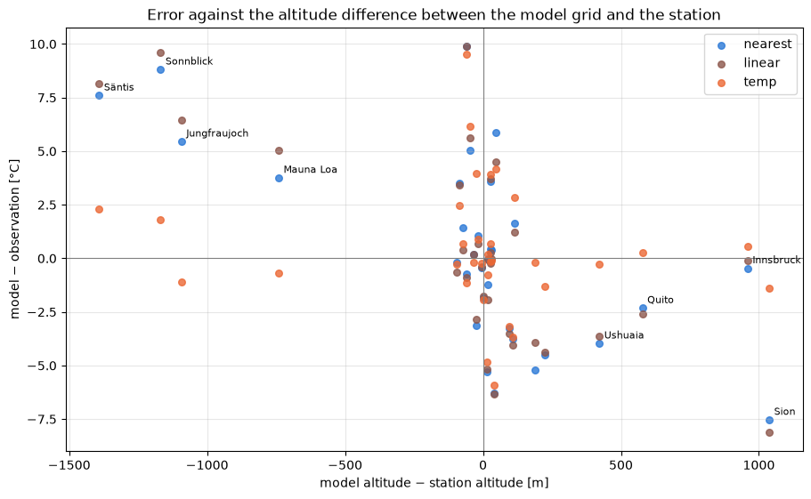
The maps show the observations and the difference between each method and the observation, on a common colour scale centred on zero. The table below lists the values per station, and the last figure relates the errors to the difference between the model altitude (at the nearest grid point) and the station altitude.

diff = pois[list(METHODS)].sub(pois["observation"], axis=0)
diff_lim = np.ceil(np.nanmax(np.abs(diff.to_numpy())))
obs_lim = np.ceil(np.nanmax(np.abs(pois["observation"])))
panels = [("observation", pois["observation"], "RdYlBu_r", -obs_lim, obs_lim)]
panels += [(f"method={label} − observation", diff[label], "RdBu_r", -diff_lim, diff_lim) for label in METHODS]

fig, axes = plt.subplots(
    2, 2, figsize=(14, 7.5), layout="constrained", subplot_kw={"projection": ccrs.Robinson(central_longitude=0)}
)
for ax, (title, values, cmap, vmin, vmax) in zip(axes.flat, panels):
    ax.set_global()
    ax.add_feature(cfeature.COASTLINE, linewidth=0.5, edgecolor="0.4")
    scatter = ax.scatter(
        pois["LONGITUDE"],
        pois["LATITUDE"],
        c=values,
        cmap=cmap,
        vmin=vmin,
        vmax=vmax,
        s=45,
        edgecolor="0.2",
        linewidth=0.4,
        transform=ccrs.PlateCarree(),
    )
    ax.set_title(title)
    if title == "observation":
        fig.colorbar(scatter, ax=ax, location="left", shrink=0.8, label="observed 2 m temperature [°C]")
fig.colorbar(scatter, ax=axes, shrink=0.6, label="model − observation [°C]")
fig.suptitle(f"GFS 0.25°, run {run:%Y-%m-%d %H} UTC, valid {valid_time:%Y-%m-%d %H:%M} UTC")
plt.show()

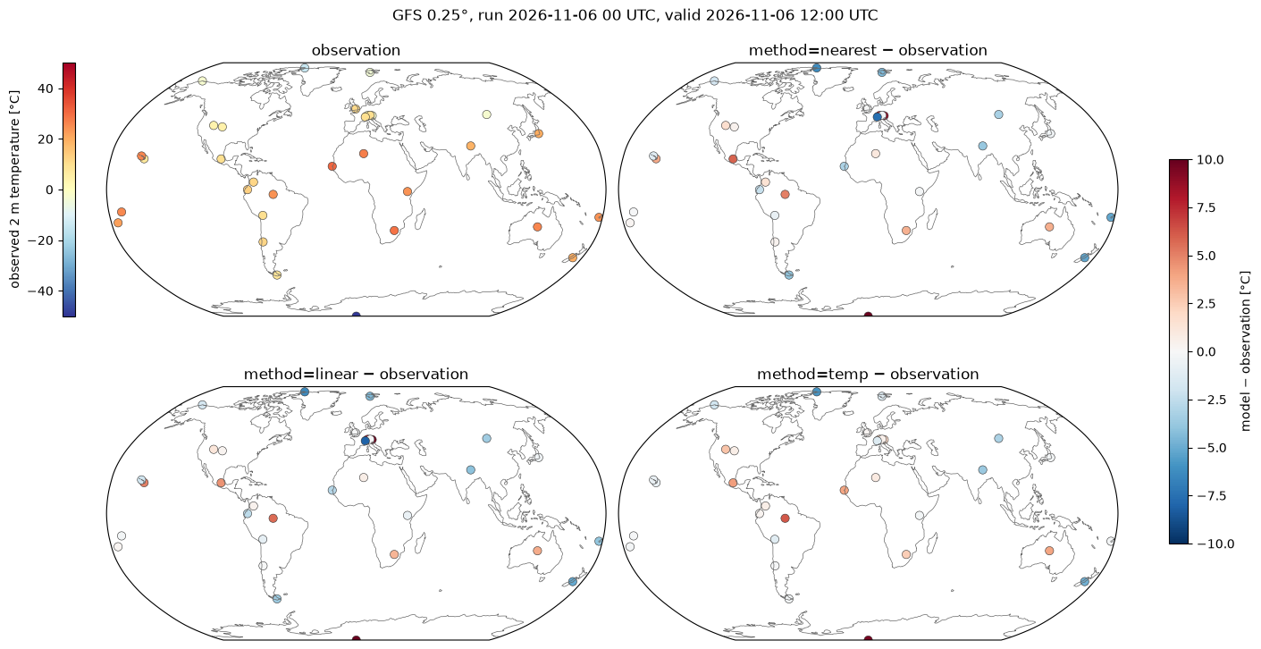
table = pois[["name", "terrain", "ELEVATION", "model altitude", "observation", *METHODS]].rename(
    columns={
        "ELEVATION": "station altitude [m]",
        "model altitude": "model altitude [m]",
        "observation": "observed [°C]",
    }
)
table = table.astype({label: "float64" for label in METHODS})  # float32 values display with spurious digits
table.round({"model altitude [m]": 0, "observed [°C]": 1, **dict.fromkeys(METHODS, 1)}).set_index("name")

	terrain	station altitude [m]	model altitude [m]	observed [°C]	nearest	linear	temp
name
Jungfraujoch	high mountain	3576.0	2483.0	-6.5	-1.0	-0.1	-7.6
Säntis	high mountain	2500.0	1108.0	-0.2	7.4	7.9	2.1
Sonnblick	high mountain	3113.8	1945.0	-2.8	6.0	6.8	-1.0
Mauna Loa	high mountain	3407.4	2667.0	7.1	10.9	12.1	6.4
El Alto	high mountain	4061.5	4002.0	10.0	9.3	9.1	8.8
Mexico City	high city	2229.9	2276.0	10.0	15.9	14.5	14.2
Bogotá	high city	2548.4	2477.0	12.0	13.4	12.4	12.7
Quito	high city	2400.0	2978.0	13.0	10.7	10.4	13.3
Nairobi	high city	1623.7	1528.0	24.0	23.8	23.4	23.7
Johannesburg	high city	1694.1	1610.0	29.0	32.5	32.4	31.5
Denver	high city	1647.1	1675.0	4.4	4.8	4.7	5.1
Salt Lake City	high city	1288.4	1404.0	3.9	5.6	5.1	6.7
Ulaanbaatar	high city	1330.1	1424.0	-3.0	-6.2	-6.5	-6.2
Tamanrasset	high city	1377.1	1360.0	27.0	28.1	27.7	27.9
Innsbruck	valley	580.9	1540.0	10.0	9.5	9.9	10.5
Sion	valley	481.9	1519.0	10.0	2.5	1.9	8.6
Kathmandu	valley	1338.1	1447.0	19.0	15.2	14.9	15.3
Santiago	valley	482.0	514.0	12.0	12.4	12.0	11.9
Nadi	coast/island	18.0	207.0	24.0	18.8	20.1	23.8
Fua'amotu	coast/island	38.4	5.0	22.0	22.2	22.2	21.8
Pago Pago	coast/island	3.7	30.0	25.7	25.6	25.5	25.6
Honolulu	coast/island	1.8	18.0	26.0	24.8	24.1	25.2
Dakar	coast/island	25.9	0.0	31.0	27.9	28.1	35.0
Tokyo	coast/island	10.7	6.0	20.0	19.6	19.6	19.8
Ushuaia	coast/island	21.6	443.0	8.0	4.0	4.4	7.7
Christchurch	coast/island	37.5	51.0	20.0	14.7	14.8	15.2
London	coast/island	25.3	43.0	11.2	11.2	11.2	11.4
Manaus	lowland/desert	68.5	21.0	24.0	29.0	29.6	30.2
Alice Springs	lowland/desert	545.3	571.0	26.0	29.6	29.7	29.9
South Pole	polar	2835.0	2775.0	-49.4	-39.5	-39.5	-39.9
Alert	polar	62.0	101.0	-14.7	-21.0	-21.0	-20.6
Utqiaġvik	polar	8.2	8.0	-3.0	-4.9	-4.7	-4.9
Longyearbyen	polar	26.8	249.0	-4.0	-8.5	-8.4	-5.3

COLORS = {"nearest": "#2a78d6", "linear": "#8c564b", "temp": "#eb6834"}

alt_diff = pois["model altitude"] - pois["ELEVATION"]
fig, ax = plt.subplots(figsize=(9, 5.5), layout="constrained")
for label in METHODS:
    ax.scatter(alt_diff, diff[label], color=COLORS[label], s=30, label=label, alpha=0.8)
for name, x, y in zip(pois["name"], alt_diff, diff["nearest"]):
    if abs(x) > 300:
        ax.annotate(name, (x, y), textcoords="offset points", xytext=(4, 4), fontsize=8)
ax.axhline(0, color="0.5", lw=0.8)
ax.axvline(0, color="0.5", lw=0.8)
ax.set_xlabel("model altitude − station altitude [m]")
ax.set_ylabel("model − observation [°C]")
ax.set_title("Error against the altitude difference between the model grid and the station")
ax.grid(alpha=0.3)
ax.legend()
plt.show()

Performance benchmark

The first call includes building the neighbor search structures, which grid_process caches. Subsequent calls on the same grid and stations (e.g. for other variables or runs) reuse them: their runtime is the mean ± standard deviation over 5 repetitions.

def benchmark(
    func: Callable[..., xr.Dataset],
    data: xr.Dataset,
    target: gpd.GeoDataFrame | xr.Dataset,
    methods: dict[str, dict[str, Any]],
    first_call_times: dict[str, float],
    repeat: int = 5,
) -> pd.DataFrame:
    """Runtime of the first call and mean ± standard deviation of the subsequent calls of each method."""
    rows: dict[str, dict[str, Any]] = {}
    for method, kw in methods.items():
        times = np.array(timeit.repeat(partial(func, data, target, **kw), number=1, repeat=repeat))
        rows[method] = {
            "first call [s]": f"{first_call_times[method]:.3f}",
            "subsequent calls [s]": f"{times.mean():.3f} ± {times.std():.3f}",
        }
    return pd.DataFrame.from_dict(rows, orient="index").rename_axis("method")


print(f"{ds.latitude.size} × {ds.longitude.size} grid points -> {len(pois)} stations")
runs = {"nearest": METHODS["nearest"], "nearest (try_reg=True)": {"method": "nearest", "try_reg": True}}
runs |= {label: kwargs for label, kwargs in METHODS.items() if label != "nearest"}
benchmark(gri.interp2poi, ds, pois, runs, first_call).rename(index={"nearest": "nearest (try_reg=False)"})

721 × 1440 grid points -> 33 stations

	first call [s]	subsequent calls [s]
method
nearest (try_reg=False)	0.627	0.165 ± 0.005
nearest (try_reg=True)	0.006	0.004 ± 0.000
linear	0.013	0.004 ± 0.000
temp	0.653	0.215 ± 0.006

Takeaways

• At 0.25° the model orography smooths out the mountains: on Säntis, Sonnblick, Jungfraujoch and Mauna Loa the nearest grid point is 700 to 1400 m below the station, and nearest and linear are about 4 to 10 °C too warm. In the valley of Sion the grid point is 1000 m above the station, and they are about 8 °C too cold. temp corrects most of these differences: its errors stay within about 2.5 °C at these stations.

• Where the model altitude is close to the station altitude, the three methods agree. The remaining differences to the observations (e.g. in Mexico City, Manaus, Christchurch or at the South Pole) come from the model itself, not from the interpolation. Observations taken up to an hour from the valid time also add some differences.

• Coastal stations are more mixed: the neighborhood of temp contains land and sea grid points. At Nadi it removes most of the error of nearest, while at Dakar it is warmer than the observation. If needed, the sea grid points can be masked, e.g. with ds.where(land_fraction > 0.5) and the GFS land-sea mask (LAND): grid points that are NaN for all variables are ignored in the neighbor search.

• The ECEF neighbor search handles the stations next to the antimeridian (Nadi, Fua’amotu, Pago Pago) and close to the poles like any other. At the South Pole, all neighbors are the same pole point repeated in the first grid row: temp cannot fit a sounding and falls back to a fixed lapse rate.

• linear is not available in ECEF: on a regular latitude/longitude grid such as GFS it goes through the regular grid interpolation (try_reg=True, the default), which also handles the 0..360° longitudes of GFS and the stations across its 360° seam.

• The first call of nearest (try_reg=False) and temp includes converting the 1 million grid points to ECEF and building the neighbor search, about 0.6 s. Subsequent calls take about 0.2 s. On a regular grid such as GFS, the regular grid interpolation (try_reg=True) is 40 to 100 times faster: nearest and linear take a few milliseconds, and nearest picks the same grid point as in ECEF at all stations. The ECEF neighbor search remains needed by the methods using a neighborhood, such as temp, and by unstructured grids.