Regridding: ERA5 2 m temperature on the global IFS 0.1° grid#

This example illustrates interp2grid() on the whole globe with three methods:

nearest: value of the nearest source grid point;
linear: bilinear interpolation on the regular latitude/longitude grid;
temp_fixgrad: among the source grid points within r_search grid spacings, the one with the most similar altitude, corrected for the remaining altitude difference with a fixed lapse rate (6 K/km by default).

The 2 m temperature of the ERA5 reanalysis (regular 0.25° grid, about 28 km, 1.04 million points) at a single time is regridded to the global 0.1° grid of the IFS open data (about 9 km, 6.5 million cells), whose orography resolves the mountains in much more detail.

Both grids are in latitude/longitude and cover the globe, so the nearest neighbor searches of nearest (with try_reg=False) and temp_fixgrad run in earth-centered earth-fixed coordinates (ECEF): distances are measured in meters through the Earth, so they are correct everywhere, across the antimeridian and at the poles.

Running this notebook needs a free account on the Copernicus Climate Data Store: your API token in ~/.cdsapirc and the licence of the ERA5 dataset accepted once on its download page. It uses about 8 GB of memory.

Data: contains modified Copernicus Climate Change Service information 2026, ERA5 hourly data on single levels (DOI: 10.24381/cds.adbb2d47), CC BY 4.0. ECMWF open data, © ECMWF, CC BY 4.0. Coastlines: Natural Earth.

import contextlib
import io
import logging
import re
import time
import timeit
from collections.abc import Callable
from functools import partial
from typing import Any

# import pyproj before earthkit.data to avoid a crash at exit (earthkit-data#1202)
import pyproj  # noqa: F401  # pylint: disable=unused-import

import cartopy.crs as ccrs
import earthkit.data as ekd
import earthkit.plots as ekp
import geopandas as gpd
import numpy as np
import pandas as pd
import requests
import xarray as xr
from requests.adapters import HTTPAdapter
from urllib3.util import Retry

import grid_process.grid_interp as gri
import grid_process.units_conv as uconv

METHODS: dict[str, dict[str, Any]] = {
    "nearest": {"method": "nearest"},
    "linear": {"method": "linear"},
    "temp_fixgrad": {"method": "temp_fixgrad"},
}
ERA5_TIME = "2025-01-15T12:00"  # single time of the ERA5 reanalysis
# zooms on mountain regions: (longitude, latitude) bounds
REGIONS = {
    "Himalaya": ((75.0, 100.0), (40.0, 25.0)),
    "Andes": ((-80.0, -60.0), (-10.0, -35.0)),
    "Alps": ((5.0, 16.5), (48.5, 43.5)),
}

Visual comparison#

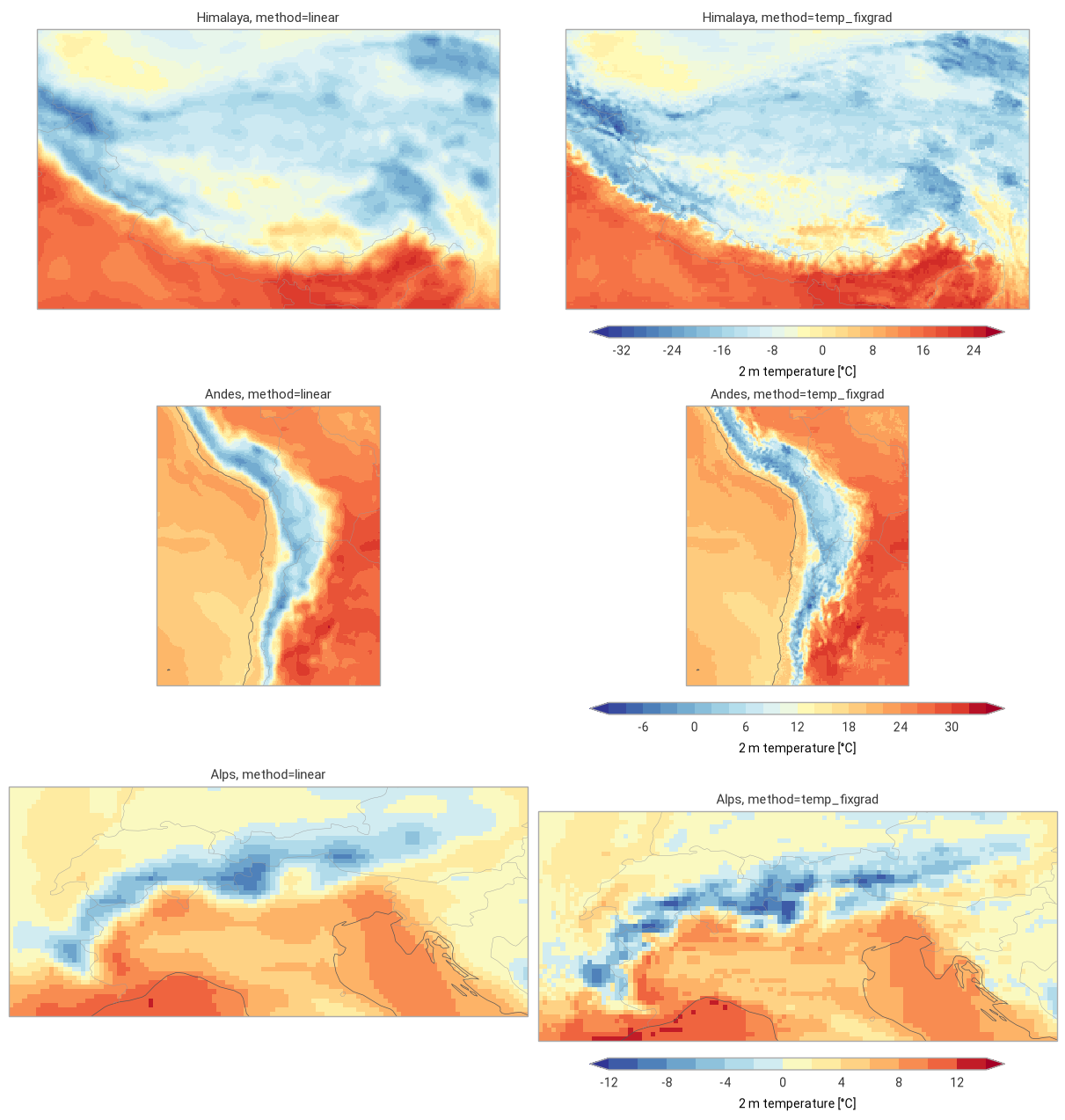
The global maps show the three methods and the correction of temp_fixgrad with respect to linear (differences below 1 °C in white). The zooms on three mountain regions compare linear and temp_fixgrad.

style = ekp.styles.Style(levels=np.arange(-50, 46, 5), colors="RdYlBu_r", extend="both", units="°C")
diff_style = ekp.styles.Style(levels=[-12, -8, -4, -2, -1, 1, 2, 4, 8, 12], colors="RdBu_r", extend="both", units="°C")
correction = results["temp_fixgrad"]["t2m"] - results["linear"]["t2m"]
panels = [(f"method={label}", results[label]["t2m"], style) for label in METHODS]
panels.append(("temp_fixgrad − linear", correction, diff_style))

fig = ekp.Figure(rows=2, columns=2, figsize=(14, 8), crs=ccrs.PlateCarree())
for i, (title, field, panel_style) in enumerate(panels):
    subplot = fig.add_map(i // 2, i % 2)
    subplot.pcolormesh(
        field.values, x=field.longitude.values, y=field.latitude.values, style=panel_style, transform=ccrs.PlateCarree()
    )
    subplot.coastlines(linewidth=0.4)
    subplot.title(title)
    subplot.legend(label="2 m temperature [°C]" if panel_style is style else "difference [°C]")
fig.title(f"ERA5 2 m temperature {ERA5_TIME.replace('T', ' ')} UTC on the IFS 0.1° grid")
fig.show()

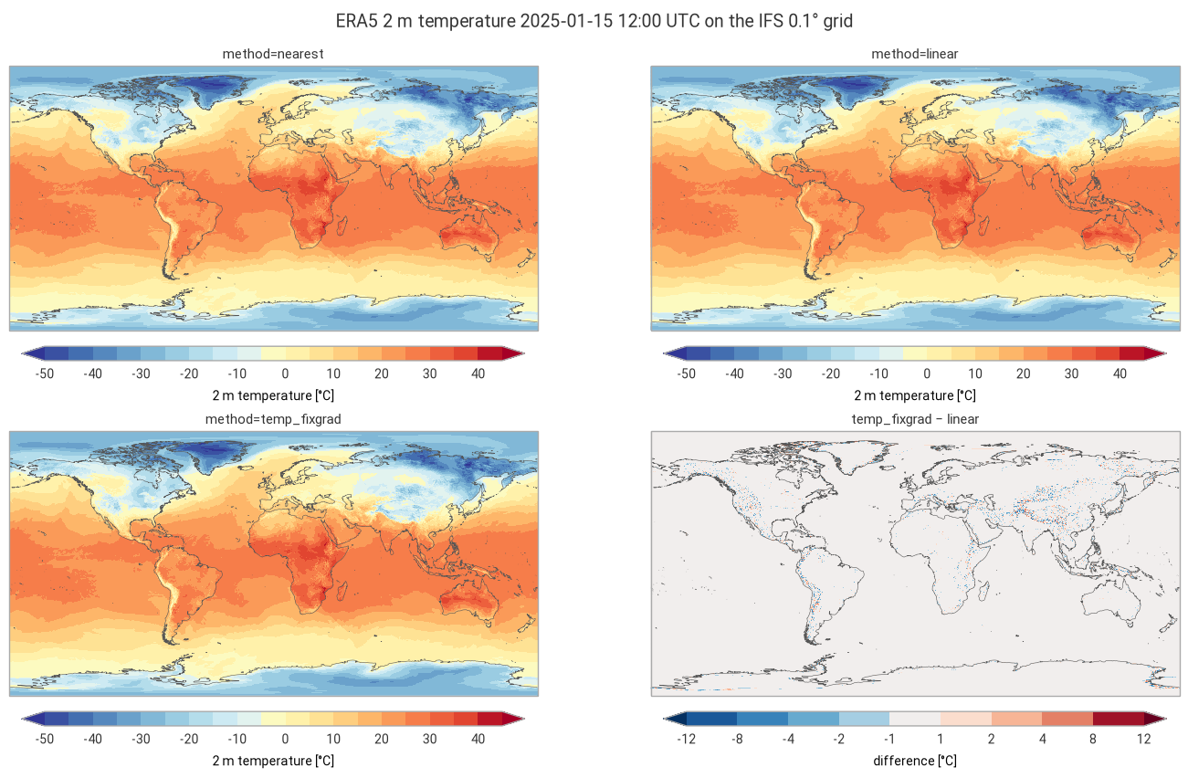
../_images/ef49f8f732d710f2412f7d7a40cb57a82b85e7bbce15b95a46111d5ba3b9078f.png

fig = ekp.Figure(rows=len(REGIONS), columns=2, figsize=(12, 4.2 * len(REGIONS)), crs=ccrs.PlateCarree())
for row, (region, (lon_bnds, lat_bnds)) in enumerate(REGIONS.items()):
    box = {"longitude": slice(*lon_bnds), "latitude": slice(*lat_bnds)}
    fields = [results[label]["t2m"].sel(box) for label in ("linear", "temp_fixgrad")]
    region_style = ekp.styles.Style(
        levels=np.arange(np.floor(min(f.min() for f in fields)), np.ceil(max(f.max() for f in fields)) + 2, 2),
        colors="RdYlBu_r",
        extend="both",
        units="°C",
    )
    for col, (label, field) in enumerate(zip(("linear", "temp_fixgrad"), fields)):
        subplot = fig.add_map(row, col)
        subplot.pcolormesh(
            field.values,
            x=field.longitude.values,
            y=field.latitude.values,
            style=region_style,
            transform=ccrs.PlateCarree(),
        )
        subplot.coastlines(linewidth=0.5)
        subplot.borders(linewidth=0.3)
        subplot.title(f"{region}, method={label}")
    subplot.legend(label="2 m temperature [°C]")
fig.show()

../_images/14e776e023ed18d03712c44cf7d7697e7dfd0ff2bb56618c8999676df9778c2b.png

Performance benchmark#

The first call includes building the neighbor search structures and converting the coordinates, which grid_process caches. Subsequent calls on the same grids (e.g. for other variables or times) reuse them: their runtime is the mean ± standard deviation over 5 repetitions.

def benchmark(
    func: Callable[..., xr.Dataset],
    data: xr.Dataset,
    target: gpd.GeoDataFrame | xr.Dataset,
    methods: dict[str, dict[str, Any]],
    first_call_times: dict[str, float],
    repeat: int = 5,
) -> pd.DataFrame:
    """Runtime of the first call and mean ± standard deviation of the subsequent calls of each method."""
    rows: dict[str, dict[str, Any]] = {}
    for method, kw in methods.items():
        times = np.array(timeit.repeat(partial(func, data, target, **kw), number=1, repeat=repeat))
        rows[method] = {
            "first call [s]": f"{first_call_times[method]:.3f}",
            "subsequent calls [s]": f"{times.mean():.3f} ± {times.std():.3f}",
        }
    return pd.DataFrame.from_dict(rows, orient="index").rename_axis("method")


print(
    f"{ds.latitude.size} × {ds.longitude.size} source grid points -> "
    f"{dst_grid.latitude.size} × {dst_grid.longitude.size} cells"
)
benchmark(gri.interp2grid, ds, dst_grid, runs, first_call)

721 × 1440 source grid points -> 1801 × 3600 cells

	first call [s]	subsequent calls [s]
method
nearest	0.034	0.020 ± 0.001
linear	0.149	0.127 ± 0.001
temp_fixgrad	7.200	3.266 ± 0.022
nearest (try_reg=False)	2.777	1.448 ± 0.003

Takeaways#

nearest and linear keep the 0.25° (28 km) structure of ERA5: they ignore the more detailed orography of the 0.1° grid. temp_fixgrad corrects for the altitude difference between the source grid point and the destination cell, which brings back the terrain: cold ridges and warmer valleys in the Himalaya, the Andes and the Alps.
The correction exceeds 1 °C in only 3 % of the cells worldwide, but in 14 to 31 % of the cells of the three mountain regions, mostly within ±5 °C. Over the oceans and plains the methods agree within about 1 °C; there temp_fixgrad takes a single source grid point, like nearest, while linear blends four.
All cells get a value with every method, including across the 360° seam of the ERA5 grid (0 to 360°) in the -180 to 180° destination grid and at the poles.
On a regular grid, nearest selects the same source point with the regular grid interpolation (try_reg=True, in degrees) and with the generic path in ECEF (try_reg=False), but about 70 times faster. The generic path is needed for the neighborhood methods (here temp_fixgrad) and irregular grids, whose neighbors must be searched in meters.
Regridding 1 million source points to 6.5 million cells takes a fraction of a second with the regular grid interpolation. The generic path converts both grids to ECEF and builds the neighbor search at the first call (about 3 s for nearest, 7 s for temp_fixgrad), which subsequent calls reuse.

Regridding: ERA5 2 m temperature on the global IFS 0.1° grid#

Destination grid#

Source data#

Interpolation#

Visual comparison#

Performance benchmark#

Takeaways#